After seeing how the rules of the physical world constrain and shape movements of real objects, it’s time to turn to the pixels. State-aware UI controls that have become pervasive in the last decade are not pure eye candy. Changing the fill / border color of a button when you move the mouse cursor over it serves as the indication that the button is ready to be pressed. Consistent and subtle visual feedback of the control state plays significant role in enabling flowing and productive user experience, and color manipulation is one of the most important techniques.

Electron gun was one of my favorite technical terms in the eighties, and i remember being distinctly impressed by the fact that any visible color can be simulated with the right mix of red, green and blue phosphor cells. Somehow, mixing equal amounts of red, green and blue blobs of play-doh always left me with a brownish green bigger blob, but the pictures on the screen were certainly colored.

If you have a few hours to kill, color theory is a topic as endless as it gets. One of the basic terms in color theory is that of chromacity – which refers to the pure hue of the color. It is usually illustrated as a tilted horse shoe, with one of the sides representing the wavelengths of the visible spectrum (image courtesy of Wikimedia):

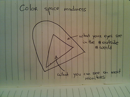
The problem is that average monitors (not only CRT, but LCD / plasmas as well) cannot reproduce the full visible spectrum. In color theory this is referred to as the color space – mathematical model that describes how colors can be represented by numbers. The sRGB color space is one of the most widely used for the consumer displays. Put simply, it is a triangle with red, green and blue points inside the chromacity graph (courtesy of Wikimedia):

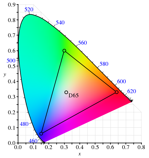
The ironic thing about this diagram is that it cannot be faithfully shown on a display that uses the sRGB color space – since it cannot reproduce any of the colors outside the inner triangle (color space in printing is an equally lengthy subject).

Now let’s see whether the constraints of the moving physical objects are relevant for animating color pixels on the screen.

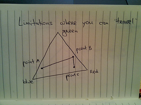
Suppose you have a button. It is displayed with light blue inner fill. When the user moves the mouse over the button (rollover), you want to animate the inner fill to yellow, and when the user presses the button, you want to animate the inner fill to saturated orange. These three colors represent anchor points of a movement path inside the specific color space:

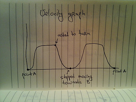
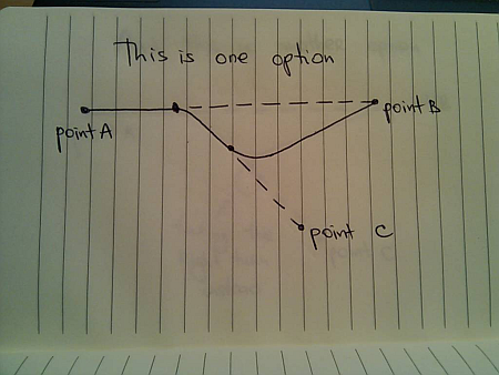
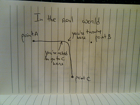
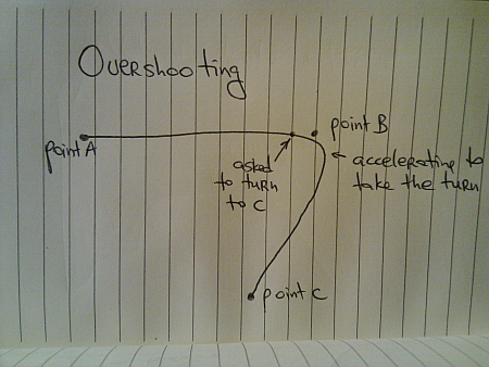
Imagine what happens when the user moves the mouse over the button, and presses it before the rollover animation has been completed. The direct analogy to the physical world is an object that was moving from point A to point B, and is now asked to turn to point C before reaching B. If the color animation reflects the momentum / inertia of the physical movement, the trajectory around point B may take the path outside the color space:

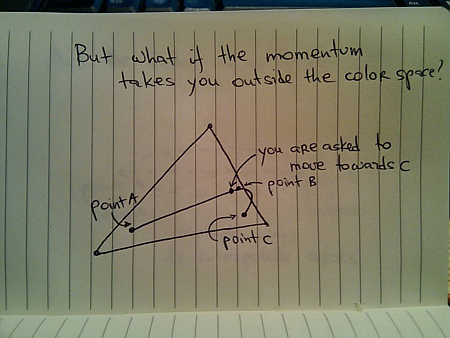
This is similar to physical world limitations – say, if point B is very close to a lake, and you don’t want to drive your new car into it. In this case you will need to clamp the interpolated color to lie inside the confines of the specific color space.

In the physical world, if you want to get from point A to point B, you would usually take the shortest route. This is not so simple if you’re interpolating colors. There’s a whole bunch of different color spaces (RGB, XYZ and HSV are just a few), and each one has its own “shortest” route that connects two colors:

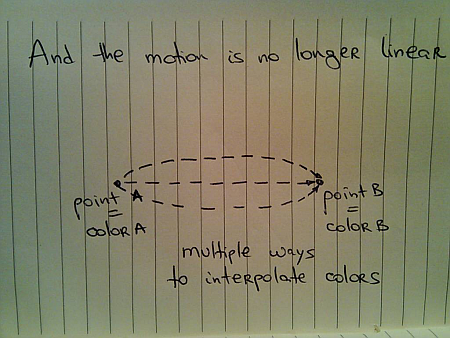
Chet’s entry from last summer has a short video and a small test application that shows the difference between interpolating colors in RGB and HSV color spaces.

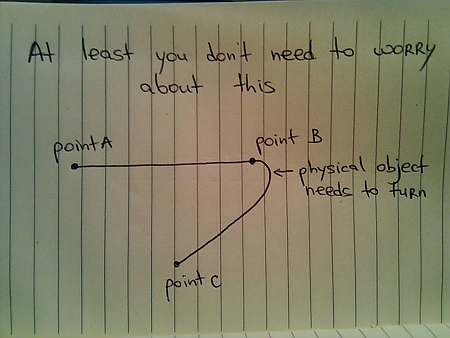
When you’re interpolating colors, the analogy to a moving physical object holds as far as the current direction, velocity and momentum. However, the moving “color object” does not have any volume – unlike the real physical objects. Thus, if it went from point A to point B (and stopped completely), and is now asked to either go back to A or go to point C, it does not need to turn – compare this to the case above when it was asked to turn to C while it was still moving towards B.

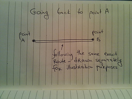
However, the rules of momentum still apply while the animation is still in progress. Suppose you’re painting your buttons with light blue color (point A) when they are inactive, and with yellow color (point B) when the mouse is over them. The user moves the mouse over one of the buttons and it starts animating – going from point A to point B. Now the user moves the mouse away from the button as it is still animating – and you want to go back to point A. If you want to follow the rules of physical movement, you cannot immediately go back from your current color back to the light blue. Rather, you need to follow the current momentum towards the yellow color, decelerate and only then go back to light blue.

Next, i’m going to talk about layout animations.

To be continued tomorrow.

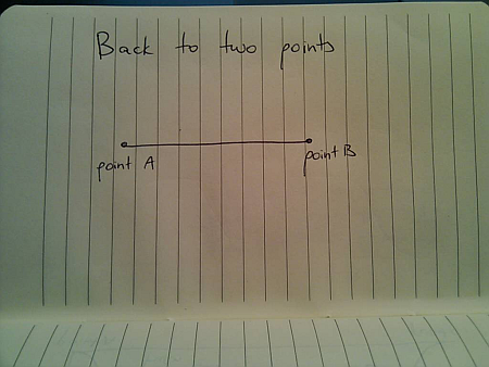
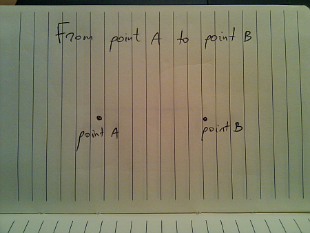
After looking at movement paths involving three points, let’s go back to the case of two points:

Now, once you arrive at B you are asked to go back to A. A straightforward solution would look like this:

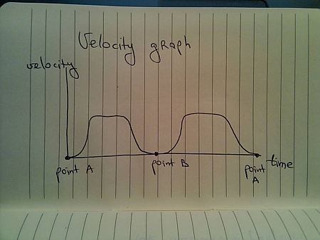
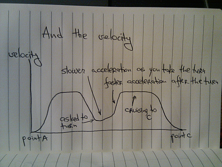
With the velocity graph for the overall travel:

What about being asked to go back to A before you get to B?

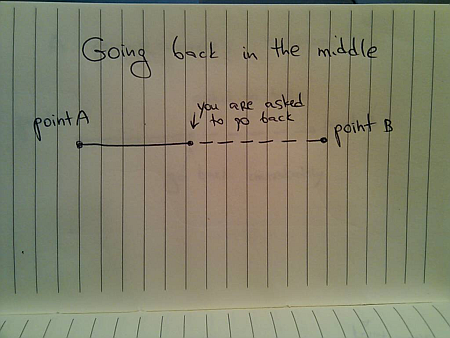
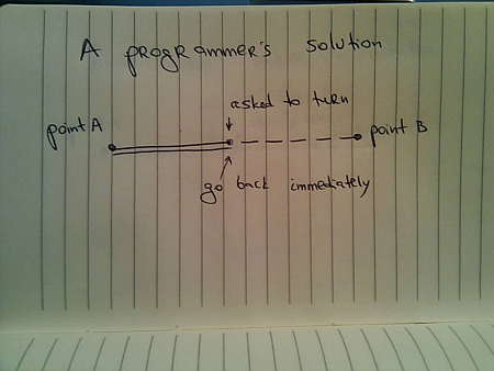
Extending the previous solution, the first approach would be

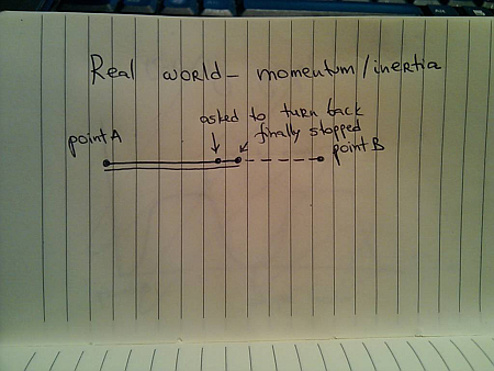
However, just as in the previous entry (with three points), when you are asked to change direction while you’re still moving, you need to account for your current momentum /inertia. In this case, it will take you some time to slow down – while still going towards B, and then you can start moving back to A:

And the corresponding velocity graph looks like this:

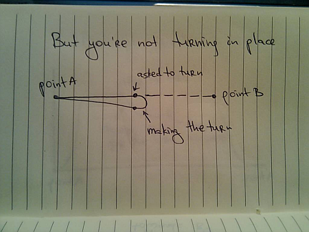
The movement paths in the previous entry remind us that the moving body is in most cases not symmetric around the Z axis, and so needs to take an actual turn – unless it’s a train bogie with driver cabs on both sides:

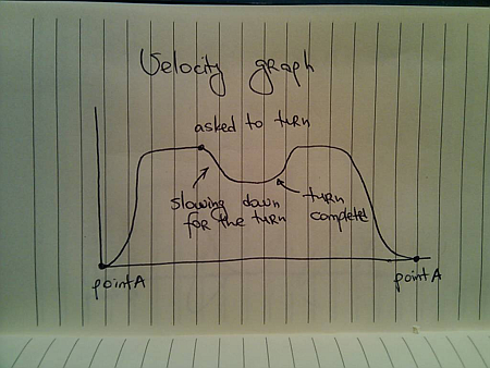
And the velocity graph with the turn does not have a zero-velocity point in the middle:

Going back to the case where you don’t need to take the turn (train bogie or other examples that will be discussed in the next installments), notice that you’re travelling more after being asked to turn back:

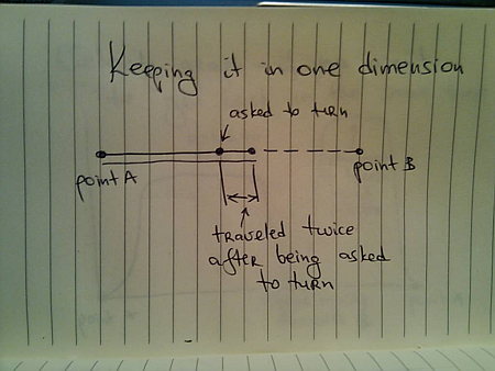
If X time units have passed since you left A and until you were asked to turn, and you are asked to get back to A in the same X time units, this means that you will need to travel faster:

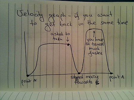
with the actual speed depending on how much does it take you to decelerate once you’ve been asked to go back, and how much distance do you have to cover before getting to A.

Now, let’s extend this example to three points:

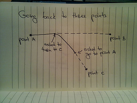
Here, you were asked to go to C while you were moving towards B, and are asked to change direction once again as you are moving towards C. The movement path will include you making a right turn towards A – creating a complex two-dimensional trajectory:

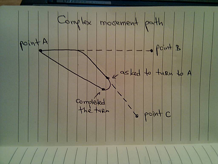
What if you’re asked to move to B instead?

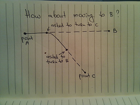
In this case you’re going to take a left turn towards B:

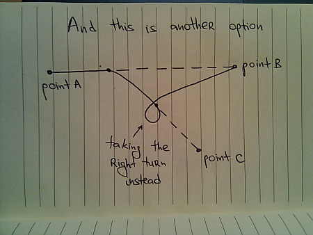
Or, if you’re a big fan of right turns (or have a problem with your steering wheel), you can take the right turn:

In any case, the real world does not have segmented paths

All the examples in this series have talked about everyday movements of physical objects. Next, i’m going to talk how the same principles apply to the objects and entities displayed on the screen.

To be continued tomorrow.

The examples in the previous entry talked about moving from point A to point B in a straight line:

Now let’s add one more point – after arriving at point B you are asked to head to point C:

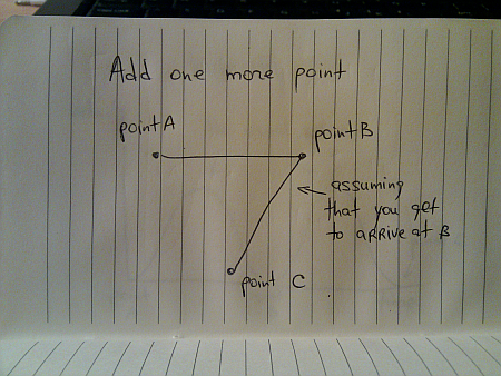
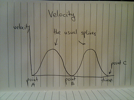
Assuming the prevalent usage of splines to approximate the acceleration and deceleration of the two segments, we have this velocity graph:

However, physical objects are not infinitely small points, and the vast majority are not perfectly symmetrical around the Z axis. To put it in a simpler term, a moving physical object has the “front” or “face” side:

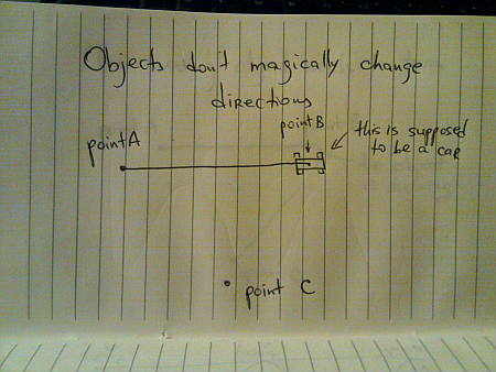
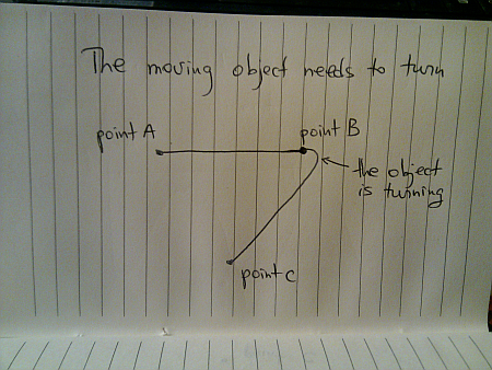
So, when the object starts moving towards C (especially if it is a man made vehicle on regular wheels), it needs to make a turn before it points to C – and can continue moving toward it in a straight line:

Even if you didn’t particularly like physics in high school, you have to deal with centrifugal force on every highway entry and exit – you have to slow down when you take the turn, otherwise your insurance policy is going to be quite expensive. On the related note – this is why outer edge of highway exits (as well as curving railroad tracks) is slightly raised.

How does the velocity graph look around point B?

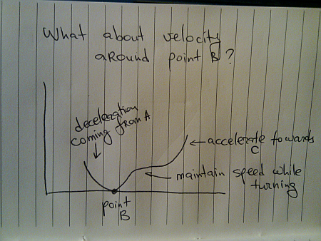
As you start turning, you accelerate until you reach speed which you deem safe to maintain as long as you are turning. Once the turn is done, you start accelerating towards the cruising speed, heading directly towards C.

Depending on what type of driver you are, you can decide to take a smaller curve and drive slower, or drive faster but take a bigger curve:

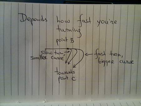
Here you can see how adding the second dimension to the movement path (since C does not lie on the line connecting A and B) adds infinite possibilities to the overall movement trajectory.

Let’s take this one step further – suppose that you are in between A and B, and are asked to move to C:

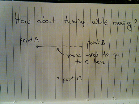
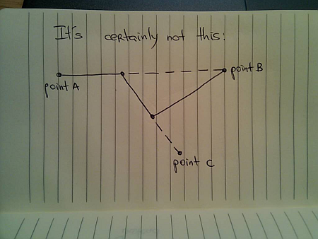
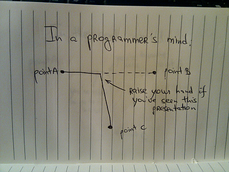
If you are on a solid plain (say, a prairie or a dry lake bed), the optimal decision is to make your turn towards C as soon as possible – without arriving at B first. Hopefully by now your solution is not going to look like this:

In the real world, you have two factors that will prevent this from happening. First one was mentioned above – most moving physical objects are not perfectly symmetrical around the Z axis and need to turn around to have their preferred movement direction aligned towards C. The second is due to the momentum, or inertia. If you are moving with non-zero speed towards point B, you cannot immediately switch the direction – just as you cannot immediately go from zero to your cruising speed.

Thus, the movement path is quite similar to the one seen above (when you move to C after arriving at B):

What about the velocity graph?

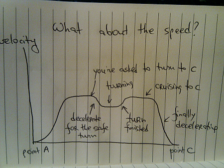
Here, you don’t need to decelerate all the way to zero speed (unless you’re a really bad driver) in order to turn your vehicle and align with C. You decelerate to your preferred turn speed, complete the turn and then accelerate back to your cruising speed (minus all the distractions along the way).

This is just one possible scenario. Here, we have been asked to turn to C while we are driving at our preferred cruising speed. What if you are asked to turn just a few moments after starting from point A – as you are still accelerating?

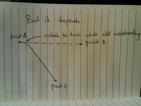
Depending on where exactly you are when this happens (specifically, whether your current speed is lower than your preferred turning speed), the velocity graph may look like this:

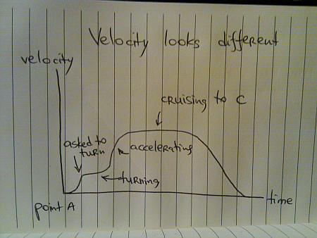
This graph assumes that you are asked to turn when you are moving at exactly your preferred turning speed. If it happens earlier, you will still be accelerating even as you begin the turn. If it happens later, you will drop your speed as you start turning, complete the turn and then accelerate towards C.

Finally, suppose you are asked to turn to C as you are decelerating and getting ready to stop at B:

Once again, depending on your current speed you will need to either decelerate or accelerate towards your preferred turning speed, complete the turn and accelerate towards C. Depending on your preferred turning speed you may even overshoot point B as you are completing the turn.

One possible velocity graph for this scenario looks like this:

Here, the assumption is that you are asked to turn when your current speed is lower than your preferred turning speed. In this case, you start accelerating as you are turning, and then complete the acceleration after the turn is done.

As before, you see and experience all of these scenarios every day. The next time you get on or off the highway, just notice all the decisions that your body is conveying to the car – and analyze the reasons behind each one of them.

To be continued tomorrow.

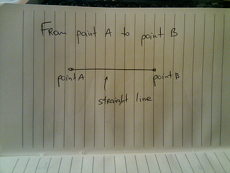
Movement is all around us in the physical world. We take it for granted since we see it from the moment we’re born. Today, i’m going to talk about a seemingly mundane act of moving from one given point to another given point. I would imagine that if you’re reading this, you most probably enjoyed your math lessons in middle school, so the following drawing should be familiar:

 

In a perfect world (imagine a deserted highway), moving from point A to point B is just following the straight line:

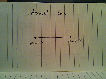
And if you’re a programmer, this is how you would implement this journey:

 

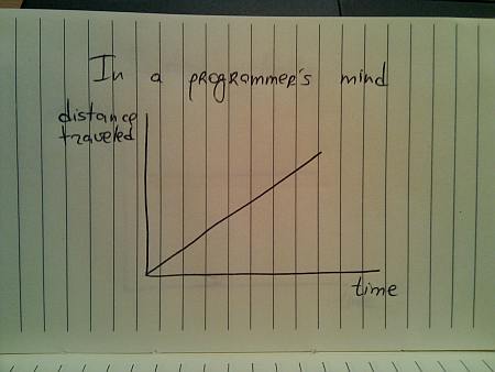
While this seems quite straightforward (and i have seen quite a few presentations that use linear animations), this falls apart once you translate the traveled distance to velocity:

 

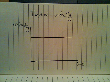
This is hardly the way things move in the real world (be they man-made, inanimate or animate). The usual approach taken by the existing animation libraries is to use a variation of spline (or perhaps a sine / cosine wave) that looks like this:

 

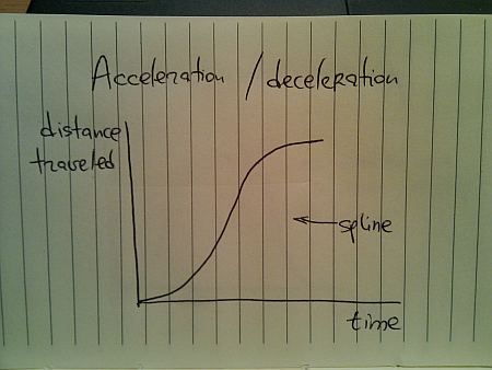
Here, you start from zero velocity, accelerate as you go, reach your maximum speed towards the middle of your journey and then start decelerating towards zero speed as you reach your destination. Translating the distance traveled to velocity, we get this:

 

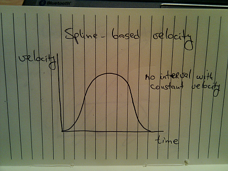
Once again, this is not how things move in the real world. A moving body (human, animal, vehicle or other) has a certain speed limit and a certain preferred speed. It takes some time to reach that speed, but once you get there, you stay until it’s time to decelerate:

 

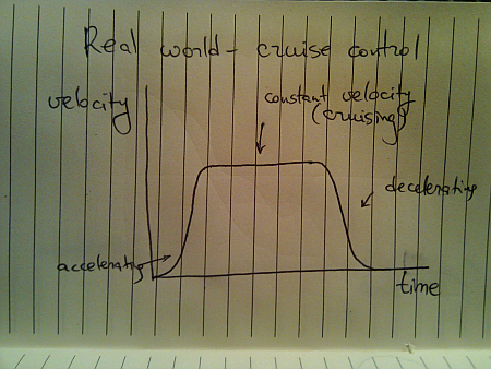
This is a better approximation of a slightly less ideal movement. The velocity graph models the “cruise control” mode that you’d employ on a deserted straight highway. Translating the velocity to distance traveled, we get this:

 

Here, we have a curving acceleration (might be a spline, a sine or even a quadratic curve – depending on the way the object is accelerating), followed by the perfectly linear segment which ends in a curving deceleration.

All the examples above assumed that you’re supposed to arrive at point B and just stop there. That is not always the case:

 

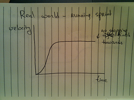
You do stop once you reach the sprint finish line, but you don’t stop until you reach it. Once you gain your maximum speed, in the ideal world you’ll be able to maintain it – especially over a very short distance.

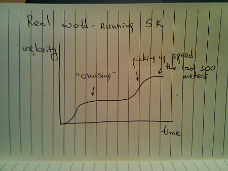
When you’re running sprint, it doesn’t really matter what are your opponents doing. They are running on parallel tracks and do not interfere with your pace. However, if you switch from running sprint to running a longer distance (say 5K), the story gets quite different, and the most common velocity graph looks like this:

 

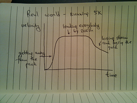
Of course, some runners try to outsmart the competition and end up running like this:

 

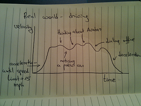
Once you leave a deserted road and have some traffic around you, you cannot always use cruise control. Even if you’re on a straight highway, your velocity graph will likely look like this:

 

Of course, these graphs are nothing new. We see countless movements of physical objects around you every day. All you need to do is look beyond the simplified approach of “train is moving with constant speed of 40mph” and start analyzing the real world.

To be continued tomorrow.