Compose Desktop gradients and Skia shaders
Drawing gradient fills is a basic tool that should be a part of every graphics framework, and Compose is not an exception. Gradients come in a variety of kinds – linear, radial, conical, sweep – each defining the “shape” of the color transition. In this post I’m going to focus on controlling the computation of intermediate colors along that shape, and as such, from this point on, I’ll only be talking about linear gradients. And more specifically, to keep the code samples focused on color interpolation, I’ll only be talking about horizontal linear gradients defined by two colors, start and end.
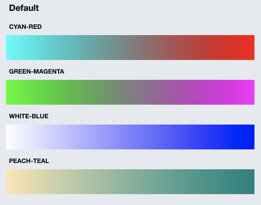
First, let’s take a look at the following screenshot:
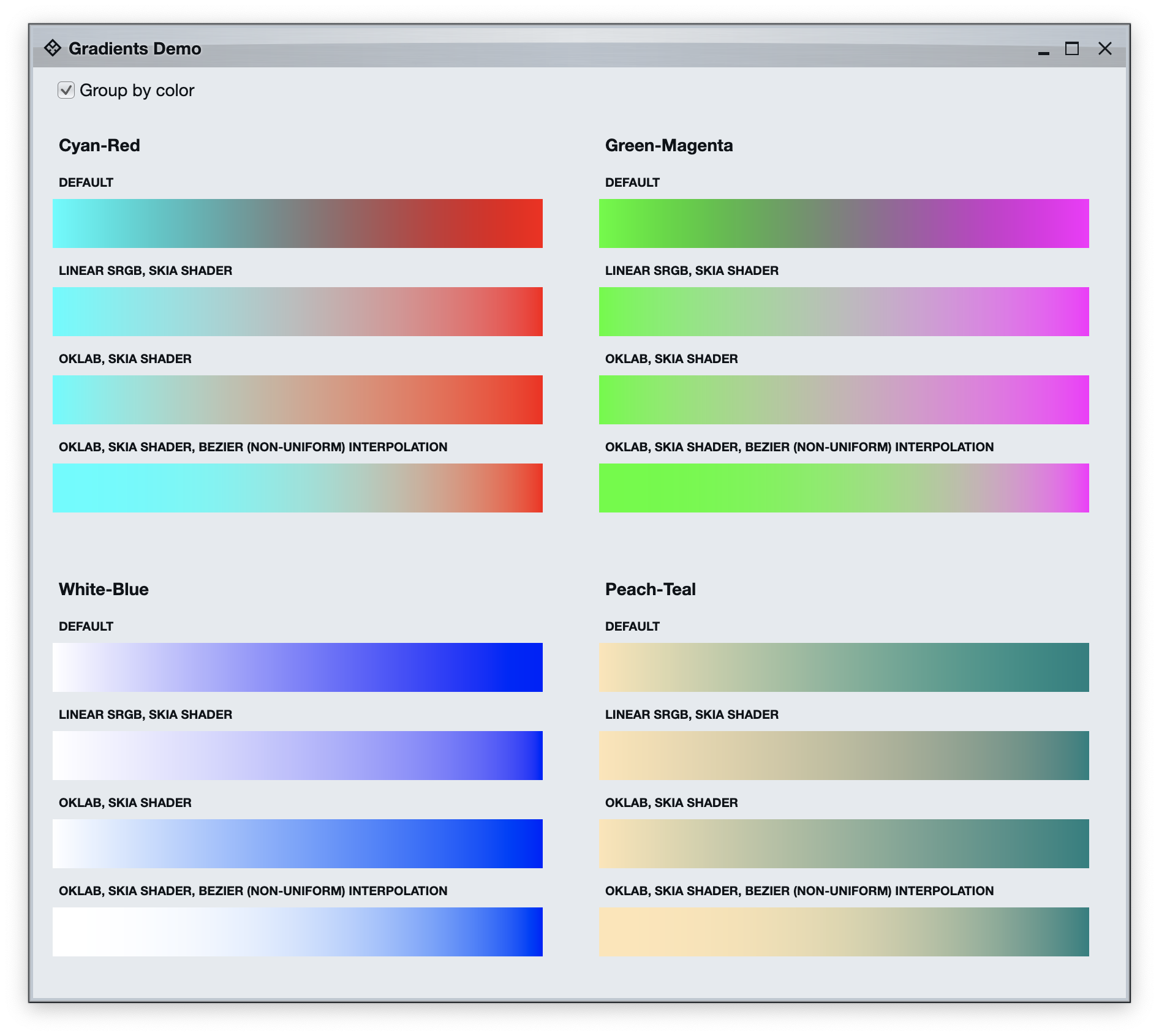
Here we have four groups of horizontal gradients. The first two are using primary colors – cyan to red and green to magenta. The third one is using white and blue. And the fourth one is using “softer” colors, in this case peach and teal. The common thing in each group is the start and end color. In each group, all the gradient rows start with the same color and end with the same color. What is different? The difference is in how we interpolate between these two colors as we “move” between these two points.
Let’s start with the default look of linear gradients provided by Compose:
It is using the Brush.horizontalGradient Compose API:
Brush.horizontalGradient(
    0.0f to colors.start,
    1.0f to colors.end,
    startX = 0.0f,
    endX = width
)
It is the simplest to use, but also the one that might result in something that doesn’t make sense. The mid-range between cyan and red is way too muddy. The mid-range between green and magenta is muddy and also has a bit of a bluish tint to it. And most of the transition from white to blue has distinct traces of purple. Why is this happening? There’s a lot of articles online that dive deep into physics of light and human perception of color, and instead of rehashing the same content, I’m going to point you to one of them.
What does it boil down to? Color spaces. A color space is a way to map colors to numbers. The default color space, aka the one used to generate the gradients above, is called sRGB or standard RGB. And it’s not best suited for color interpolation, especially when our start and end colors are not similar – such as cyan and red that have drastically different hue, or white and blue that have drastically different brightness.
If we want our gradient transitions to be closer to physical light blending in real world, or closer to how human eye perceives color transitions, we need to explore other color spaces. At the present moment, even though Compose supports a wide variety of color spaces, it does not provide APIs to configure which color space to use for a specific Brush-created gradient.
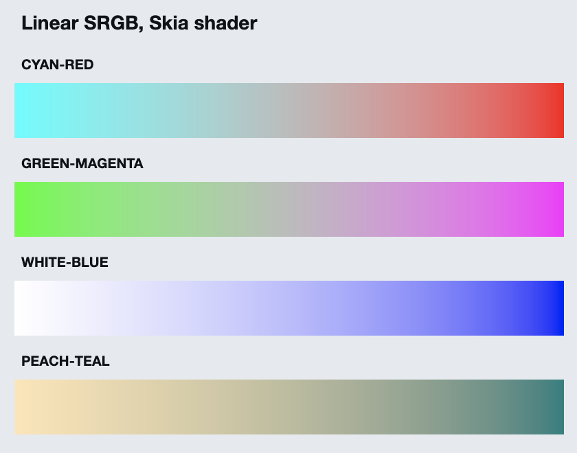
However, that should not stop us from dropping to a lower level and continuing the exploration of Skia shaders in Compose Desktop, this time for more fine-grained control of our gradients. Let’s start with Linear sRGB color space which will get us much closer to how light behaves physically:
val sksl = """
    // https://bottosson.github.io/posts/colorwrong/#what-can-we-do%3F
    vec3 linearSrgbToSrgb(vec3 x) {
        vec3 xlo = 12.92*x;
        vec3 xhi = 1.055 * pow(x, vec3(1.0/2.4)) - 0.055;
        return mix(xlo, xhi, step(vec3(0.0031308), x));

    }

    vec3 srgbToLinearSrgb(vec3 x) {
        vec3 xlo = x / 12.92;
        vec3 xhi = pow((x + 0.055)/(1.055), vec3(2.4));
        return mix(xlo, xhi, step(vec3(0.04045), x));
    }

    uniform vec4 start;
    uniform vec4 end;
    uniform float width;

    half4 main(vec2 fragcoord) {
       // Implicit assumption in here that colors are full opacity
       float fraction = fragcoord.x / width;
       // Convert start and end colors to linear SRGB
       vec3 linearStart = srgbToLinearSrgb(start.xyz);
       vec3 linearEnd = srgbToLinearSrgb(end.xyz);
       // Interpolate in linear SRGB space
       vec3 linearInterpolated = mix(linearStart, linearEnd, fraction);
       // And convert back to SRGB
       return vec4(linearSrgbToSrgb(linearInterpolated), 1.0);
    }
"""

val dataBuffer = ByteBuffer.allocate(36).order(ByteOrder.LITTLE_ENDIAN)
// RGBA colorLight
dataBuffer.putFloat(0, colors.start.red)
dataBuffer.putFloat(4, colors.start.green)
dataBuffer.putFloat(8, colors.start.blue)
dataBuffer.putFloat(12, colors.start.alpha)
// RGBA colorDark
dataBuffer.putFloat(16, colors.end.red)
dataBuffer.putFloat(20, colors.end.green)
dataBuffer.putFloat(24, colors.end.blue)
dataBuffer.putFloat(28, colors.end.alpha)
// Width
dataBuffer.putFloat(32, width)

val effect = RuntimeEffect.makeForShader(sksl)
val shader = effect.makeShader(
    uniforms = Data.makeFromBytes(dataBuffer.array()),
    children = null,
    localMatrix = null,
    isOpaque = false
)

ShaderBrush(shader)
What are we doing here? It’s a three-step process:
- Convert the start and end colors to the Linear sRGB color space. Remember that a color space is a way to map colors to numbers. What we’re doing here is mapping our colors to a different set of numbers.
- Do linear interpolation between the converted colors based on the X coordinate.
- Convert the interpolated color back to the sRGB color space.
Let’s see the end result again
Here we see most of the muddiness gone between cyan and red, and green and magenta – even though we are losing some of the vibrancy in that transition, especially in green-magenta. And we still have a distinct purple hue in the white-blue gradient.
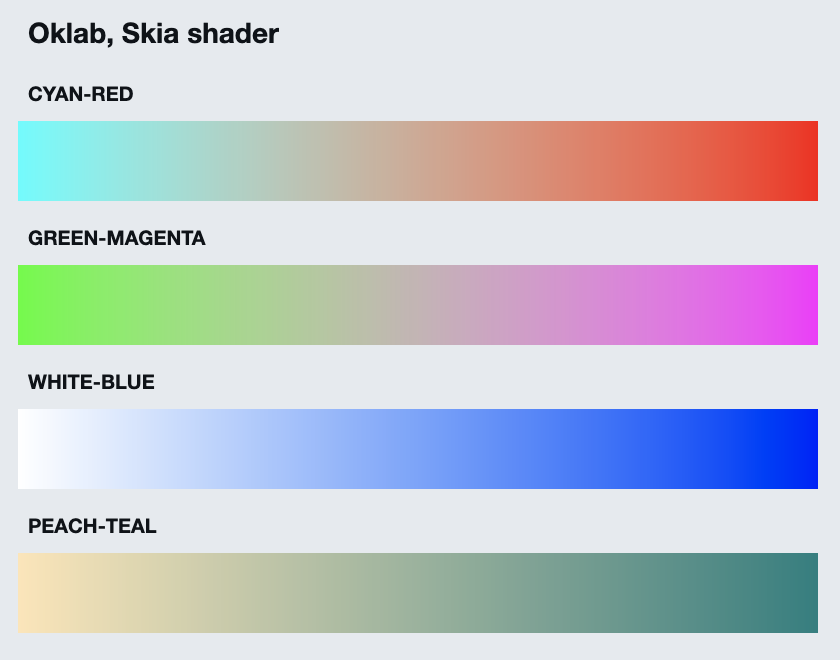
And now it’s time to look at Oklab, a recent project that aims to provide a perceptually uniform color space. Here are our gradients under Oklab:
val sksl = """
    // https://bottosson.github.io/posts/colorwrong/#what-can-we-do%3F
    vec3 linearSrgbToSrgb(vec3 x) {
        vec3 xlo = 12.92*x;
        vec3 xhi = 1.055 * pow(x, vec3(1.0/2.4)) - 0.055;
        return mix(xlo, xhi, step(vec3(0.0031308), x));

    }

    vec3 srgbToLinearSrgb(vec3 x) {
        vec3 xlo = x / 12.92;
        vec3 xhi = pow((x + 0.055)/(1.055), vec3(2.4));
        return mix(xlo, xhi, step(vec3(0.04045), x));
    }

    // https://bottosson.github.io/posts/oklab/#converting-from-linear-srgb-to-oklab
    const mat3 fromOkStep1 = mat3(
       1.0, 1.0, 1.0,
       0.3963377774, -0.1055613458, -0.0894841775,
       0.2158037573, -0.0638541728, -1.2914855480);

    const mat3 fromOkStep2 = mat3(
       4.0767416621, -1.2684380046, -0.0041960863,
       -3.3077115913, 2.6097574011, -0.7034186147,
       0.2309699292, -0.3413193965,  1.7076147010);

    const mat3 toOkStep1 = mat3(
       0.4122214708, 0.2119034982, 0.0883024619,
       0.5363325363, 0.6806995451, 0.2817188376,
       0.0514459929, 0.1073969566, 0.6299787005);

    const mat3 toOkStep2 = mat3(
       0.2104542553, 1.9779984951, 0.0259040371,
       0.7936177850, -2.4285922050, 0.7827717662,
       -0.0040720468, 0.4505937099, -0.8086757660);

    vec3 linearSrgbToOklab(vec3 x) {
        vec3 lms = toOkStep1 * x;
        return toOkStep2 * (sign(lms)*pow(abs(lms), vec3(1.0/3.0)));
    }

    vec3 oklabToLinearSrgb(vec3 x) {
        vec3 lms = fromOkStep1 * x;
        return fromOkStep2 * (lms * lms * lms);
    }

    uniform vec4 start;
    uniform vec4 end;
    uniform float width;

    half4 main(vec2 fragcoord) {
       // Implicit assumption in here that colors are full opacity
       float fraction = fragcoord.x / width;
       // Convert start and end colors to Oklab
       vec3 oklabStart = linearSrgbToOklab(srgbToLinearSrgb(start.xyz));
       vec3 oklabEnd = linearSrgbToOklab(srgbToLinearSrgb(end.xyz));
       // Interpolate in Oklab space
       vec3 oklabInterpolated = mix(oklabStart, oklabEnd, fraction);
       // And convert back to SRGB
       return vec4(linearSrgbToSrgb(oklabToLinearSrgb(oklabInterpolated)), 1.0);
    }
"""

val dataBuffer = ByteBuffer.allocate(36).order(ByteOrder.LITTLE_ENDIAN)
// RGBA colorLight
dataBuffer.putFloat(0, colors.start.red)
dataBuffer.putFloat(4, colors.start.green)
dataBuffer.putFloat(8, colors.start.blue)
dataBuffer.putFloat(12, colors.start.alpha)
// RGBA colorDark
dataBuffer.putFloat(16, colors.end.red)
dataBuffer.putFloat(20, colors.end.green)
dataBuffer.putFloat(24, colors.end.blue)
dataBuffer.putFloat(28, colors.end.alpha)
// Width
dataBuffer.putFloat(32, width)

val effect = RuntimeEffect.makeForShader(sksl)
val shader = effect.makeShader(
    uniforms = Data.makeFromBytes(dataBuffer.array()),
    children = null,
    localMatrix = null,
    isOpaque = false
)

ShaderBrush(shader)
It’s the same three-step process that we had with the Linear sRGB:
- Convert the start and end colors to the Oklab color space. Note that if you’re operating in N color spaces and need to convert colors between any two arbitrary color spaces, it is easier to designate one of them as intermediary. In our case, we transform from sRGB to Linear sRGB, and then from Linear sRGB to Oklab.
- Do linear interpolation between the converted colors based on the X coordinate.
- Convert the interpolated color back to the sRGB color space (via Linear sRGB).
Let’s see the end result again
Most of the muddiness gone between cyan and red, and green and magenta is still gone, but now we also have a bit more vibrancy in that transition, especially in cyan-red. And our white-blue gradient does not have any presence of that purple hue that we saw in sRGB and Linear sRGB gradients.
Now, since we are in control of how each pixel gets its color, we can go a bit deeper. Up until now, the interpolation step itself is doing a simple linear computation. A point halfway between the start and the end gets 50% of each component (which might be red/green/blue in sRGB, or something a bit more “abstract” in other color spaces). What if we wanted to a non-uniform interpolation on our target color space, something that, let’s say, favors the start point so that its color spreads deeper into the final gradient?
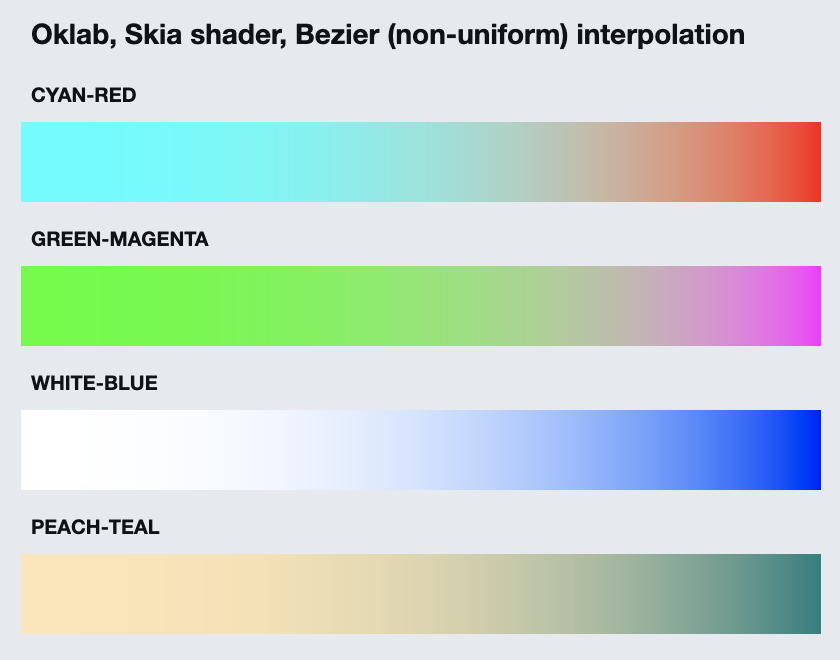
Staying in the Oklab color space, let’s switch from uniform interpolation between start and end colors to use a custom Bezier curve:
val sksl = """
    // https://bottosson.github.io/posts/colorwrong/#what-can-we-do%3F
    vec3 linearSrgbToSrgb(vec3 x) {
        vec3 xlo = 12.92*x;
        vec3 xhi = 1.055 * pow(x, vec3(1.0/2.4)) - 0.055;
        return mix(xlo, xhi, step(vec3(0.0031308), x));

    }

    vec3 srgbToLinearSrgb(vec3 x) {
        vec3 xlo = x / 12.92;
        vec3 xhi = pow((x + 0.055)/(1.055), vec3(2.4));
        return mix(xlo, xhi, step(vec3(0.04045), x));
    }

    // https://bottosson.github.io/posts/oklab/#converting-from-linear-srgb-to-oklab
    const mat3 fromOkStep1 = mat3(
       1.0, 1.0, 1.0,
       0.3963377774, -0.1055613458, -0.0894841775,
       0.2158037573, -0.0638541728, -1.2914855480);

    const mat3 fromOkStep2 = mat3(
       4.0767416621, -1.2684380046, -0.0041960863,
       -3.3077115913, 2.6097574011, -0.7034186147,
       0.2309699292, -0.3413193965,  1.7076147010);

    const mat3 toOkStep1 = mat3(
       0.4122214708, 0.2119034982, 0.0883024619,
       0.5363325363, 0.6806995451, 0.2817188376,
       0.0514459929, 0.1073969566, 0.6299787005);

    const mat3 toOkStep2 = mat3(
       0.2104542553, 1.9779984951, 0.0259040371,
       0.7936177850, -2.4285922050, 0.7827717662,
       -0.0040720468, 0.4505937099, -0.8086757660);

    vec3 linearSrgbToOklab(vec3 x) {
        vec3 lms = toOkStep1 * x;
        return toOkStep2 * (sign(lms)*pow(abs(lms), vec3(1.0/3.0)));
    }

    vec3 oklabToLinearSrgb(vec3 x) {
        vec3 lms = fromOkStep1 * x;
        return fromOkStep2 * (lms * lms * lms);
    }

    // https://en.wikipedia.org/wiki/B%C3%A9zier_curve
    vec2 spline(vec2 start, vec2 control1, vec2 control2, vec2 end, float t) {
        float invT = 1.0 - t;
        return start * invT * invT * invT + control1 * 3.0 * t * invT * invT + control2 * 3.0 * t * t * invT + end * t * t * t;
    }

    uniform vec4 start;
    uniform vec4 end;
    uniform float width;

    // Bezier curve points. Note the the first control point is intentionally
    // outside the 0.0-1.0 x range to further "favor" the curve towards the start
    vec2 bstart = vec2(0.0, 0.0);
    vec2 bcontrol1 = vec2(1.3, 0.0);
    vec2 bcontrol2 = vec2(0.9, 0.1);
    vec2 bend = vec2(1.0, 1.0);

    half4 main(vec2 fragcoord) {
       // Implicit assumption in here that colors are full opacity
       float fraction = spline(bstart, bcontrol1, bcontrol2, bend, fragcoord.x / width).y;
       // Convert start and end colors to Oklab
       vec3 oklabStart = linearSrgbToOklab(srgbToLinearSrgb(start.xyz));
       vec3 oklabEnd = linearSrgbToOklab(srgbToLinearSrgb(end.xyz));
       // Interpolate in Oklab space
       vec3 oklabInterpolated = mix(oklabStart, oklabEnd, fraction);
       // And convert back to SRGB
       return vec4(linearSrgbToSrgb(oklabToLinearSrgb(oklabInterpolated)), 1.0);
    }
"""

val dataBuffer = ByteBuffer.allocate(36).order(ByteOrder.LITTLE_ENDIAN)
// RGBA colorLight
dataBuffer.putFloat(0, colors.start.red)
dataBuffer.putFloat(4, colors.start.green)
dataBuffer.putFloat(8, colors.start.blue)
dataBuffer.putFloat(12, colors.start.alpha)
// RGBA colorDark
dataBuffer.putFloat(16, colors.end.red)
dataBuffer.putFloat(20, colors.end.green)
dataBuffer.putFloat(24, colors.end.blue)
dataBuffer.putFloat(28, colors.end.alpha)
// Width
dataBuffer.putFloat(32, width)

val effect = RuntimeEffect.makeForShader(sksl)
val shader = effect.makeShader(
    uniforms = Data.makeFromBytes(dataBuffer.array()),
    children = null,
    localMatrix = null,
    isOpaque = false
)

ShaderBrush(shader)
The only difference here is in these lines:
    // Bezier curve points. Note the the first control point is intentionally
    // outside the 0.0-1.0 x range to further "favor" the curve towards the start
    vec2 bstart = vec2(0.0, 0.0);
    vec2 bcontrol1 = vec2(1.3, 0.0);
    vec2 bcontrol2 = vec2(0.9, 0.1);
    vec2 bend = vec2(1.0, 1.0);

    half4 main(vec2 fragcoord) {
       float fraction = spline(bstart, bcontrol1, bcontrol2, bend, fragcoord.x / width).y;
       ...
    }
We’re still using the X coordinate, but now we feed that into a Bezier cubic curve that heavily favors the start point (see the curve graph here). The end result is a set of gradients that have more “presence” of the start color:
To sum it all up, here are all the gradients grouped by color space and interpolation function:
A couple of notes:
- The default sRGB and the Linear sRGB color spaces are particularly bad for gradients that have a large variance in hue and / or brightness. If your gradients use perceptually close colors, such as slight variations of the same palette color, you might not need the overhead of dropping down to Skia shaders.
- Sometimes the difference between Linear sRGB and Oklab is going to be subjective, such as the peach-teal gradient above.
- The implementation above only works for horizontal, two-stop gradients. A more generic, multi-stop linear gradient that supports arbitrary direction of the gradient would need a more generic implementation.
- For radial, sweep and conical gradients, the core logic of converting colors between color spaces stays the same. The only difference is going to be how [X,Y] coordinates of a pixel are used to compute the blend factor.
And here, it’s time to say goodbye to 2021. Stay tuned for more explorations of Skia shaders in Compose Desktop in 2022!