I don’t like programming puzzles. If a small piece of code does not do what it appears to be doing after skimming through it, it is either the problem in the code itself, or the underlying libraries that it is using. Code should be easy to read, and easy to understand. This is why i didn’t enjoy any of the “Java puzzles” sessions during the last few JavaOne conferences. I have the original book and i’ve seen the presentation slides. Personally, i don’t think that i can learn much from them – except seeing that the puzzles originate from the intricacies of the language specification, unfortunate naming of the core APIs, or the artificial restrictions of binary compatibility that resulted in the mess that is core Java generics.
Unfortunately, all of these are still part of the platform – whether we want them or not. Which is why i’d like to present you with this simple Swing program based on the code from QStorm in one of the Substance forums. Note that the following code does not use Substance and runs under the default look-and-feel.
public class Puzzle1 {
   public static void main(String[] args) {
      SwingUtilities.invokeLater(new Runnable() {
         public void run() {
            JFrame frame = new JFrame("Puzzle 1");
            frame.setSize(new Dimension(300, 200));
            frame.setLocationRelativeTo(null);
            frame.setDefaultCloseOperation(JFrame.EXIT_ON_CLOSE);

            final JTable table = new JTable();
            table.getSelectionModel().addListSelectionListener(
                  new ListSelectionListener() {
                     @Override
                     public void valueChanged(ListSelectionEvent e) {
                        if (e.getValueIsAdjusting())
                           return;

                        System.out.println("Table: "
                              + table.getRowCount() + ", model: "
                              + table.getModel().getRowCount());
                     }
                  });
            table.setAutoCreateRowSorter(true);
            table.setModel(new DefaultTableModel(
                  new Object[][] { new Object[] { "Steven", 10 } },
                  new Object[] { "Name", "Value" }));
            frame.add(table, BorderLayout.CENTER);

            JPanel controls = new JPanel(
                  new FlowLayout(FlowLayout.TRAILING));

            JButton selectAllRowsBtn = new JButton("Select all rows");
            selectAllRowsBtn.addActionListener(new ActionListener() {
               public void actionPerformed(ActionEvent e) {
                  table.selectAll();
               }
            });
            controls.add(selectAllRowsBtn);

            JButton resetModelBtn = new JButton("Reset model");
            resetModelBtn.addActionListener(new ActionListener() {
               public void actionPerformed(ActionEvent e) {
                  table.setModel(new DefaultTableModel());
               }
            });
            controls.add(resetModelBtn);

            frame.add(controls, BorderLayout.SOUTH);

            frame.setVisible(true);
         }
      });
   }
}
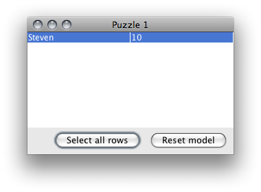
This is how the UI looks like – it has a table with one row, and two buttons on the bottom:

When the “Select all rows” button is clicked, the JTable.selectAll() is called:

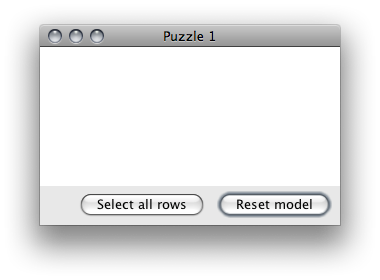
When the “Reset model” is called, the table model is reset to an empty model (no rows):

After the table is created, a selection listener is added to it. It prints the number of table rows as returned by JTable.getRowCount() and as returned by JTable.getModel().getRowCount().
What is the last line printed to the console after the two buttons have been activated?
- Table: 0, model: 0
- Table: 1, model: 0
- Table: 1, model: 1
- None of the above
Live wallpapers are now part of the officially supported APIs in Android SDK 2.1, and today i’m going to talk about how to start writing your own live wallpaper. By the end of this tutorial you should be able to create your own live wallpaper, test it on a Nexus One device and get it ready for publishing on the Android Market.
Getting started
The plumbing
The SDK comes with a sample live wallpaper that can be found in the platforms/android-2.1/samples/CubeLiveWallpaper folder. As with any other Android application, you will need to write a few XML files that let the market / device know whether your application can be run on the specific device. In our case, live wallpapers are supported by the 2.1 version of the platform, and as such should not be visible when you are browsing the market on pre-2.1 devices.
We start with the AndroidManifest.xml that looks like this:
Important points:
- The service tag lets the platform know that your service is a wallpaper
- The uses-sdk tag lets the platform know that you are requiring the 2.1 version
- The uses-feature tag lets the platform know that this is a live wallpaper
The android:resource attribute of the meta-data tag in the service description points to the bokeh.xml file that goes under the res/xml folder. Here are the contents of that file:
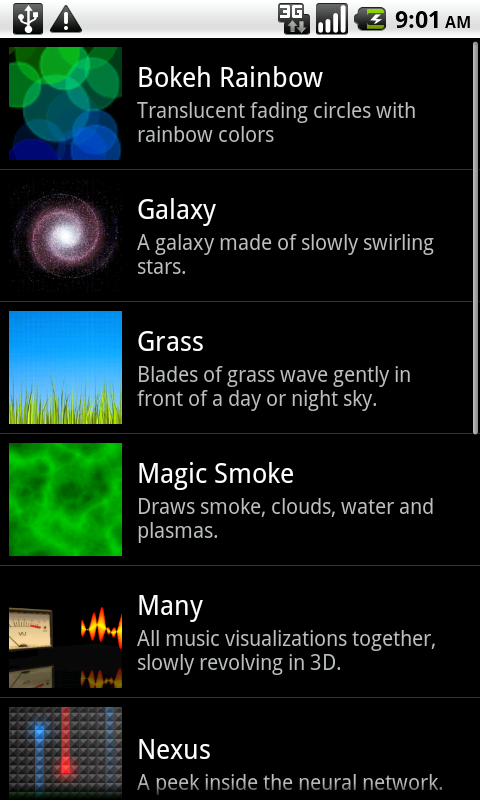
Here is how the live wallpaper picker looks like with our wallpaper at the top:
 There are two strings and one image:
- The title string is defined by the android:label attribute in the service tag of the application defined in the AndroidManifest.xml
- The description string is defined by the android:description attribute in the wallpaper defined in the bokeh.xml
- The thumbnail is defined by the android:thumbnail attribute in the wallpaper defined in the bokeh.xml
Here are the contents of res/values/strings.xml:
    Bokeh Wallpapers


    Bokeh Rainbow

    Translucent fading circles with rainbow colors
And the thumbnail image goes into the res/drawable folder.
How a live wallpaper works
A live wallpaper consists of three main layers:
- Life cycle events – create, destroy, move, show, hide, touch
- Animations
- Drawing
The android:name attribute in your service tag should point to a class name that extends the android.service.wallpaper.WallpaperService class. This is the base class for all live wallpapers in the system. It is an abstract class and you must implement the onCreateEngine() method to return your own live wallpaper engine. The engine is responsible for handling all the functionality mentioned above – life cycle events, animations and drawing.
The android.service.wallpaper.WallpaperService.Engine internal class has a number of methods that you can override in order to respond to different life cycle events of the your live wallpaper. Let’s take a short look at the relevant methods:
- onCreate() – called when the engine is initialized. At this point the drawing surface has not yet been created
- onDestroy() – called when the engine is destroyed. After this method is called, the engine is no longer valid
- onSurfaceCreated() – called when the drawing surface has been created
- onSurfaceChanged() – called when structural changes (such as size or format) have been made to the drawing surface
- onSurfaceDestroyed() – called when the drawing surface has been destroyed
- onVisibilityChanged() – called when the wallpaper becomes visible or hidden. When the wallpaper is hidden, you should suspend your animation and not draw anything to save the CPU cycles
- onOffsetsChanged() – called when the wallpaper offsets are changed after the user “swipes” the home screen to one of the sides. Can be used to create a “parallax” effect when the wallpaper is moving along with the home screen
- onTouchEvent() – called when the user performs touch-screen interaction with the window that is showing the wallpaper
- onCommand() – called to process a command
A live wallpaper is supposed to have dynamic content (hence the word “live”). The base classes (WallpaperService and WallpaperService.Engine) do not provide any special facilities to run the animation loop. It is your responsibility to start the animation loop, handle the life cycle events to suspend / resume the animations and handle each animation step. One way to handle the animation loop is with the android.os.Handler and java.lang.Runnable classes.
Let’s see a sample base implementation of an animation loop for a live wallpaper that handles the relevant events:
import android.os.Handler;
import android.service.wallpaper.WallpaperService;
import android.view.SurfaceHolder;

public abstract class AnimationWallpaper extends WallpaperService {

   protected abstract class AnimationEngine extends Engine {
      private Handler mHandler = new Handler();

      private Runnable mIteration = new Runnable() {
         public void run() {
            iteration();
            drawFrame();
         }
      };

      private boolean mVisible;

      @Override
      public void onDestroy() {
         super.onDestroy();
         // stop the animation
         mHandler.removeCallbacks(mIteration);
      }

      @Override
      public void onVisibilityChanged(boolean visible) {
         mVisible = visible;
         if (visible) {
            iteration();
            drawFrame();
         } else {
            // stop the animation
            mHandler.removeCallbacks(mIteration);
         }
      }

      @Override
      public void onSurfaceChanged(SurfaceHolder holder, int format,
            int width, int height) {
         iteration();
         drawFrame();
      }

      @Override
      public void onSurfaceDestroyed(SurfaceHolder holder) {
         super.onSurfaceDestroyed(holder);
         mVisible = false;
         // stop the animation
         mHandler.removeCallbacks(mIteration);
      }

      @Override
      public void onOffsetsChanged(float xOffset, float yOffset,
            float xOffsetStep, float yOffsetStep, int xPixelOffset,
            int yPixelOffset) {
         iteration();
         drawFrame();
      }

      protected abstract void drawFrame();

      protected void iteration() {
         // Reschedule the next redraw in 40ms
         mHandler.removeCallbacks(mIteration);
         if (mVisible) {
            mHandler.postDelayed(mIteration, 1000 / 25);
         }
      }
   }
}
Here, we have an abstract extension of the WallpaperService that handles the major life cycle events of our live wallpaper:
- The mIteration runnable will be called at each iteration to draw one single frame and schedule the next iteration
- The mHandler will handle the message queue associated with our main thread. We will use it to wait for the next iteration and run our mIteration
- The mVisible stores the current visibility flag of our wallpaper
- When the animation needs to stop – in onDestroy(), onSurfaceDestroyed() and onVisibilityChanged() when false is passed – we let our handler know that it should not run our callback. This effectively stops our animation loop, removing the animation / redraw requests.
- When the wallpaper becomes visible – in onVisibilityChanged() when true is passed, we run a single iteration and draw a single frame. The call to iteration() effectively schedules the next iteration to run in 40 milliseconds.
- Whenever there are changes to the surface – in onSurfaceChanged() and onOffsetsChanged() we respond immediately by redrawing the wallpaper and rescheduling the next iteration
Finally, it’s time to talk about the drawing. The drawFrame() method defined in our abstract class is called on every animation step. Here is how it looks like:
@Override
protected void drawFrame() {
   SurfaceHolder holder = getSurfaceHolder();

   Canvas c = null;
   try {
      c = holder.lockCanvas();
      if (c != null) {
         draw(c);
      }
   } finally {
      if (c != null)
         holder.unlockCanvasAndPost(c);
   }
}
Here, we obtain the Canvas object from the SurfaceHolder, perform the actual drawing and then unlock the canvas and let the platform know that it should draw the contents of the canvas back on the screen.
Handling the details
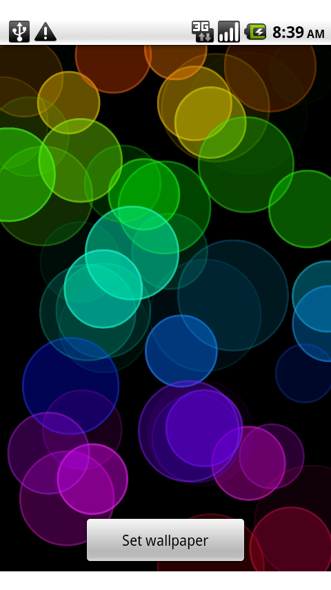
With our base abstract class handling the life cycle events and scheduling the animation iterations, we can focus on the specifics of our live wallpaper. This is how it is going to look like:
 It is a bunch of fading translucent circles that are colored based on their vertical location on the screen. First, let’s see the model class that stores the information on one single circle and updates it on every animation tick:
public class BokehRainbowCircle {
   float origRadius, deltaRadius, radius;

   float origX, deltaX, x;

   float origY, deltaY, y;

   int color;

   int alpha;

   int steps;

   int currentStep;

   public BokehRainbowCircle(float xCenter, float yCenter, float radius,
         int color, int steps) {
      this.x = xCenter;
      this.origX = xCenter;
      this.deltaX = (float) (40.0 * Math.random() - 20.0);

      this.y = yCenter;
      this.origY = yCenter;
      this.deltaY = (float) (40.0 * Math.random() - 20.0);

      this.origRadius = radius;
      this.radius = radius;
      this.deltaRadius = 0.5f * radius;

      this.color = color;
      this.alpha = 0;

      this.steps = steps;
   }

   void tick() {
      this.currentStep++;

      float fraction = (float) this.currentStep / (float) this.steps;

      this.radius = this.origRadius + fraction * this.deltaRadius;
      this.x = this.origX + fraction * this.deltaX;
      this.y = this.origY + fraction * this.deltaY;

      this.alpha = (fraction <= 0.25f) ? (int) (128 * 4.0f * fraction) : (int) (-128 * (fraction - 1) / 0.75f);
   }

   boolean isDone() {
       return this.currentStep > this.steps;
   }
}
Here, the tick() method is called on every animation iteration. This method updates the circle alpha, radius and center position to create a fading, growing and moving circle – that still maintains its color.
Now let’s see the implementation of the wallpaper itself. We start by implementing the onCreateEngine to return our own engine (note how both the wallpaper and its engine extend our base classes):
public class BokehRainbowWallpaper extends AnimationWallpaper {

   @Override
   public Engine onCreateEngine() {
      return new BokehEngine();
   }

   class BokehEngine extends AnimationEngine {
As mentioned before, the home screen (of at least Nexus One) can be swiped to the side (left or right). The wallpaper can respond to these events and create a parallax effect – where it shifts with the home screen, but at a lesser extent. In this specific case, our live wallpaper is twice as wide as the visible width of the screen. Since Nexus One can be scrolled by two screens to both sides, this creates a nice effect whereby the wallpaper is scrolled slower than the home screen contents, making it appear farther away from the user.
The information about the current size and offsets of the wallpaper is stored in the following fields:
int offsetX;
int offsetY;
int height;
int width;
int visibleWidth;
And set in the following life cycle events of our engine:
@Override
public void onSurfaceChanged(SurfaceHolder holder, int format,
      int width, int height) {

   this.height = height;
   if (this.isPreview()) {
      this.width = width;
   } else {
      this.width = 2 * width;
   }
   this.visibleWidth = width;

   for (int i = 0; i < 20; i++) {
      this.createRandomCircle();
   }

   super.onSurfaceChanged(holder, format, width, height);
}

@Override
public void onOffsetsChanged(float xOffset, float yOffset,
      float xOffsetStep, float yOffsetStep, int xPixelOffset,
      int yPixelOffset) {
   // store the offsets
   this.offsetX = xPixelOffset;
   this.offsetY = yPixelOffset;

   super.onOffsetsChanged(xOffset, yOffset, xOffsetStep, yOffsetStep,
         xPixelOffset, yPixelOffset);
}
Note how in onSurfaceChanged we compute the overall width of the wallpaper based on its preview state (you cannot swipe in preview mode). The offsets stored in the onOffsetsChanged are used during the drawing - see the calls to drawCircle below:
void draw(Canvas c) {
   c.save();
   c.drawColor(0xff000000);

   synchronized (circles) {
      for (BokehRainbowCircle circle : circles) {
         if (circle.alpha == 0)
            continue;

         // intersects with the screen?
         float minX = circle.x - circle.radius;
         if (minX > (-this.offsetX + this.visibleWidth)) {
            continue;
         }
         float maxX = circle.x + circle.radius;
         if (maxX < -this.offsetX) {
            continue;
         }

         paint.setAntiAlias(true);

         // paint the fill
         paint.setColor(Color.argb(circle.alpha, Color
               .red(circle.color), Color.green(circle.color),
               Color.blue(circle.color)));
         paint.setStyle(Paint.Style.FILL_AND_STROKE);
         c.drawCircle(circle.x + this.offsetX, circle.y
               + this.offsetY, circle.radius, paint);

         // paint the contour
         paint.setColor(Color.argb(circle.alpha, 63 + 3 * Color
               .red(circle.color) / 4, 63 + 3 * Color
               .green(circle.color) / 4, 63 + 3 * Color
               .blue(circle.color) / 4));
         paint.setStyle(Paint.Style.STROKE);
         paint.setStrokeWidth(3.0f);
         c.drawCircle(circle.x + this.offsetX, circle.y
               + this.offsetY, circle.radius, paint);
      }
   }

   c.restore();
}
In addition to handling the wallpaper offsets, our drawing also checks whether the specific circle needs to be painted at all. Since our wallpaper is twice as wide as the visible width of the screen, we do not need to draw those circles that lie completely to the left and to the right of the visible portion. This way we can save CPU cycle and make the wallpaper animation smoother.
The circles are created in two places. First, we create 20 circles in the onSurfaceChanged method shown above. Also, we create a circle every time the user touches the screen. This is done in the onCommand method:
@Override
public Bundle onCommand(String action, int x, int y, int z,
      Bundle extras, boolean resultRequested) {
   if ("android.wallpaper.tap".equals(action)) {
      createCircle(x - this.offsetX, y - this.offsetY);
   }
   return super.onCommand(action, x, y, z, extras, resultRequested);
}
Note the name of the command action and the usage of the offsets to create the model circle at the correct absolute location (so that when it's drawn with the offsets, it will appear at the touch spot).
Now let's take a look what happens on every animation iteration. We override the iteration() method from our super class and:
- Let each circle know that another iteration is done
- Remove all circles that have completed their life (so that our model does not grow indefinitely)
- Call the super implementation to schedule the next iteration
@Override
protected void iteration() {
   synchronized (circles) {
      for (Iterator it = circles.iterator(); it
            .hasNext();) {
         BokehRainbowCircle circle = it.next();
         circle.tick();
         if (circle.isDone())
            it.remove();
      }
      iterationCount++;
      if (isPreview() || iterationCount % 2 == 0)
         createRandomCircle();
   }

   super.iteration();
}
To complete the code, here is how we create a single model circle:
@Override
public Bundle onCommand(String action, int x, int y, int z,
      Bundle extras, boolean resultRequested) {
   if ("android.wallpaper.tap".equals(action)) {
      createCircle(x - this.offsetX, y - this.offsetY);
   }
   return super.onCommand(action, x, y, z, extras, resultRequested);
}
void createRandomCircle() {
   int x = (int) (width * Math.random());
   int y = (int) (height * Math.random());
   createCircle(x, y);
}

int getColor(float yFraction) {
   return Color.HSVToColor(new float[] { 360.0f * yFraction, 1.0f,
         1.0f });
}

void createCircle(int x, int y) {
   float radius = (float) (40 + 20 * Math.random());

   float yFraction = (float) y / (float) height;
   yFraction = yFraction + 0.05f - (float) (0.1f * (Math.random()));
   if (yFraction < 0.0f)
      yFraction += 1.0f;
   if (yFraction > 1.0f)
      yFraction -= 1.0f;
   int color = getColor(yFraction);

   int steps = 40 + (int) (20 * Math.random());
   BokehRainbowCircle circle = new BokehRainbowCircle(x, y, radius,
         color, steps);
   synchronized (this.circles) {
      this.circles.add(circle);
   }
}
The color of the circle is based on its vertical position (matching the hue to the Y fraction). The circle radius and time-to-live are computed randomly.
Packaging and testing
If you are developing your live wallpaper in Eclipse, the ADT plugin will create an .apk - Android Package file - for you. It will be under the bin folder of your project. At this point you can use the Android Debug Bridge - adb tool - to put your live wallpaper on the device and test it. Run the adb install or adb install -r (if you're replacing the existing one) command pointing to your APK file. Once your package has been installed, bring the live wallpaper picker and click on your wallpaper. Now you can test your wallpaper in both preview and live mode.
Once you are satisified with your wallpaper, it's time to sign and publish it on the Market. Congratulations! You are done.
Resources and conclusion
Complete sources and resources for this wallpaper are available on GitHub. This wallpaper is also available as a free download on the Android Market - search for "Bokeh Rainbow".
A few final words about the performance of live wallpapers. Remember that this is a mobile device, and it is not as powerful as your average laptop / desktop machine. This applies to CPU as well as memory. The more you want to put on the screen, the less fluid your wallpaper will feel. Right now the code above is using the Canvas APIs to paint the circles, and the performance is not as smooth as i would like it to be - even when i only paint the circles that intersect with the visible part of the screen. There are a few options to improve the performance.
One option is to use pre-computed bitmaps and some sort of home-grown double buffering with offscreen bitmaps. However, using a lot of bitmaps may lead to OutOfMemoryErrors - depending on how much memory is available to your process in specific, and to the system in general. You can also play with different Canvas APIs and see which ones are faster for your specific visuals. OpenGL is another option - if you feel adventurous enough.
The Developer Resources has a few articles related to performance, especially on avoiding memory leaks and tracking memory allocations. In particular, it is recommended to reuse as many instances as possible to avoid costly garbage collection of small objects - like is done with the Paint instance in the code above.
